Tutorials#
This tutorial demonstrates how to use visco for compressing and decompressing radio interferometric data. We generate a Measurement Set (MS) and synthetic visibilities using simms and MeqTrees, respectively.
Tutorial 1: Compressing and Decompressing KAT-7 Visibility Data#
Simulation setup#
The KAT-7 telescope is simulated for a 1-hour observation, using an integration time of 2 seconds.
The starting frequency is 1.4 GHz, with 64 channels, each having a width of 100 kHz.
The visibilities are simulated for a source at the phase centre that is unpolarized, with a total intensity of 1 Jy.
The visibilities are simulated with noise.
The full rank of the data is \(\min(\mathrm{timeslots}, \mathrm{channels}) = 64\).
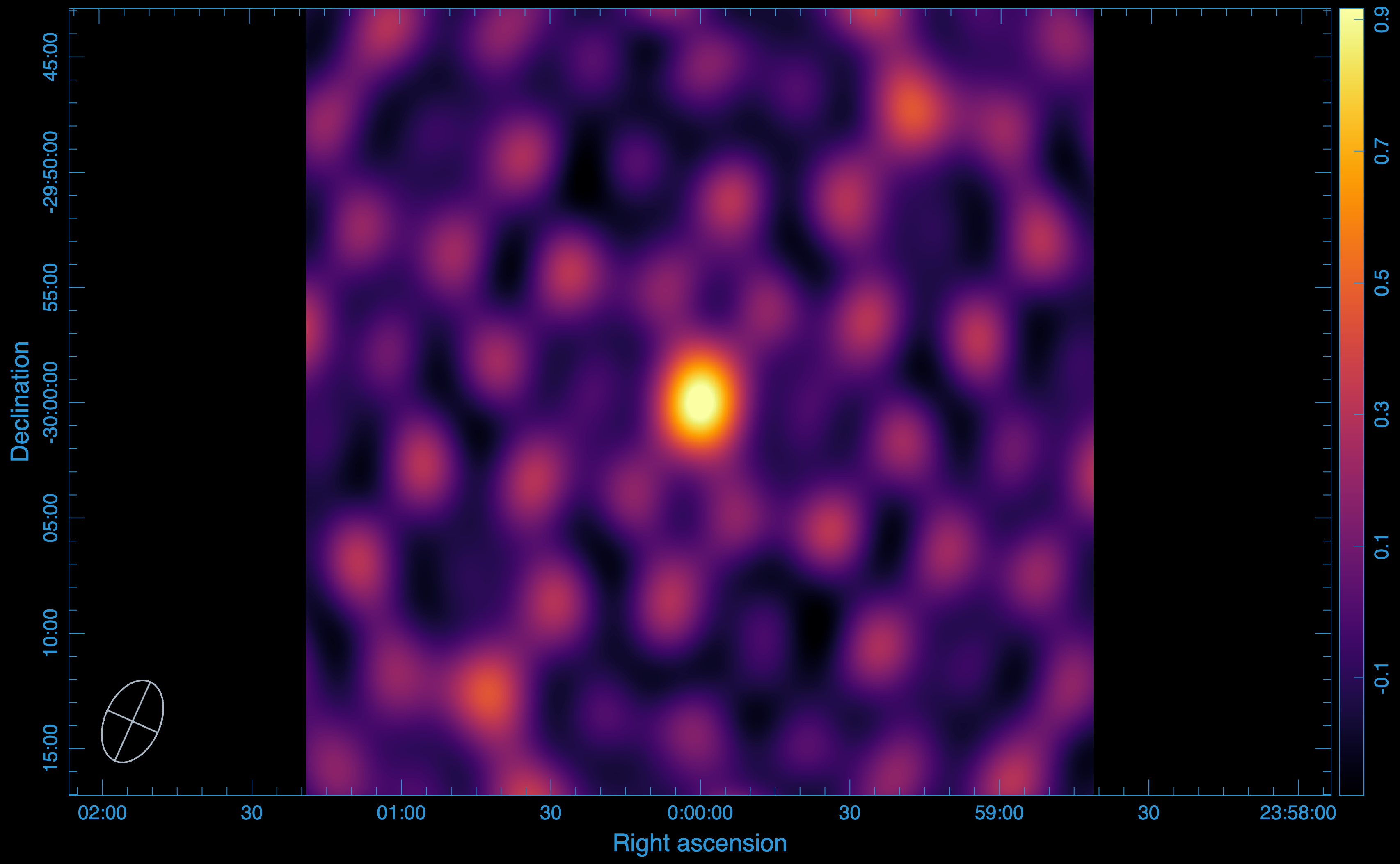
Data image:
The data image is produced using WSClean.

Note
Dirty images are used here because compression can affect the Point Spread Function (PSF).
Statistics:
We use CARTA to open the images and measure the statistics:
Peak flux: (\(1.000429391861 \times 10^{0}\)) Jy/beam
RMS: (\(1.439807312603 \times 10^{-1}\)) Jy/beam
SNR: 7
Disk usage:
The MS occupies 228 MB of disk storage.
Compressing the Visibility Data#
Now, we use visco compression functionality to compress the visibility data using singular value decomposition (SVD). SVD decomposes the visibility data for each baseline and correlation into three matrix components, U,S, and W. These three components are stored in a Zarr store. To compress the visibility data, run:
visco compressms -ms kat7-sim.ms/ -zs kat7-sim.zarr -col DATA -corr XX,XY,YX,YY -cr 1 -nw 8 -nt 1 -ml 4GB -da 2727 -csr 3600
where:
-ms gives the path to the measurement set to compress,
-zs specifies the output Zarr store path,
-col specifies the column containing the visibility data,
-corr defines the correlations to compress,
-cr is the desired compression rank,
-nw sets the number of Dask workers,
-nt specifies the number of threads per worker,
-ml sets the memory limit,
-da is the dashboard address,
-csr is the chunk size along the row.
The flag -cr 1 signifies that the data is compressed using only the first singular value or a comression rank of 1 (reducing the data rank to 1). This means that only the compnents of U and W corresponding to the first (highest) value of S are kept in the Zarr store. To see how the compression impacts the data, we have to decompress the data from the Zarr store back into an MS. To do this, we use the decompression functionality of visco.
Decompressing the data from Zarr to MS#
To decompress the data from a zarr store back into an MS for imaging, run:
visco decompressms -zs kat7-sim.zarr/ -ms kat7-sim-decompressed.ms
where:
-zp provides the path to the Zarr store containing the compressed data,
-ms sets the output MS file.
Imaging the compressed Data:
After decompressing the data, we turn to WSClean again to image the data. The output image we get is:
Statistics:
Peak flux: (\(1.000427842140 \times 10^{0}\)) Jy/beam
RMS: (\(1.439824590852 \times 10^{-1}\)) Jy/beam
SNR: 7
Smearing:
To see the imapct of compression, the most useful test to perform is to measure the level of smearing incurred by the compression. After compression, more than 99.99% of the peak flux from the original image is recovered, therefore, there is no smearing incurred by the compression.
Disk usage:
The Zarr store containing the compressed visibility data, along with the rest of the MS data, occupies only 15 MB, representing a compression factor of 15.
Tutorial 2: Improving Compression Speed using Correlations#
Compressing the visibility data using SVD is computationally expensive. Futhermore, the process is performed for each baseline and correlation product. To reduce the computational cost, you can choose to combine correlations. This approach speeds up the compression by grouping the XX & YY and XY & YX correlations together.
Although our simulation so far includes an unpolarized source where the XY and YX correlations contribute minimally, we can still test this approach. To do so, we simply add the --correlation-optimized flag to our run:
visco compressms -ms kat7-sim.ms/ -zs kat7-sim.zarr -col DATA -corr XX,XY,YX,YY -cr 1 -nw 8 -nt 1 -ml 4GB -da 2727 -csr 3600 --correlation-optimized
Data image:
We have included the –correlation-optimized flag, which let us speed up the compression process, in the run. To see the impact of the compression, we, as previously, decompress the data from the zarr store back to an MS. The image produced from this process is:

Statistics:**
Peak flux: (\(1.000429391861 \times 10^{0}\)) Jy/beam
RMS: (\(1.439828319666 \times 10^{-1}\)) Jy/beam
SNR: 7
Smearing:
We note here, too, that there is no smearing effects incurred by the compression.
Disk usage:
This method further reduces the disk storage occupied by the zarr store, with only 9 MB occupied. The compression factor achieved is 25.
Tutorial 3: Compressing and Decompressing MeerKAT Visibility Data#
Now, lets focus on the MeerKAT telescope.
Simulation setup#
We use the same simulation settings we used for the KAT-7.
Our sky model now includes 10 unpolarized point sources, each with a total intensiy of 1 Jy
Data image:
For this simulation, we get this image:
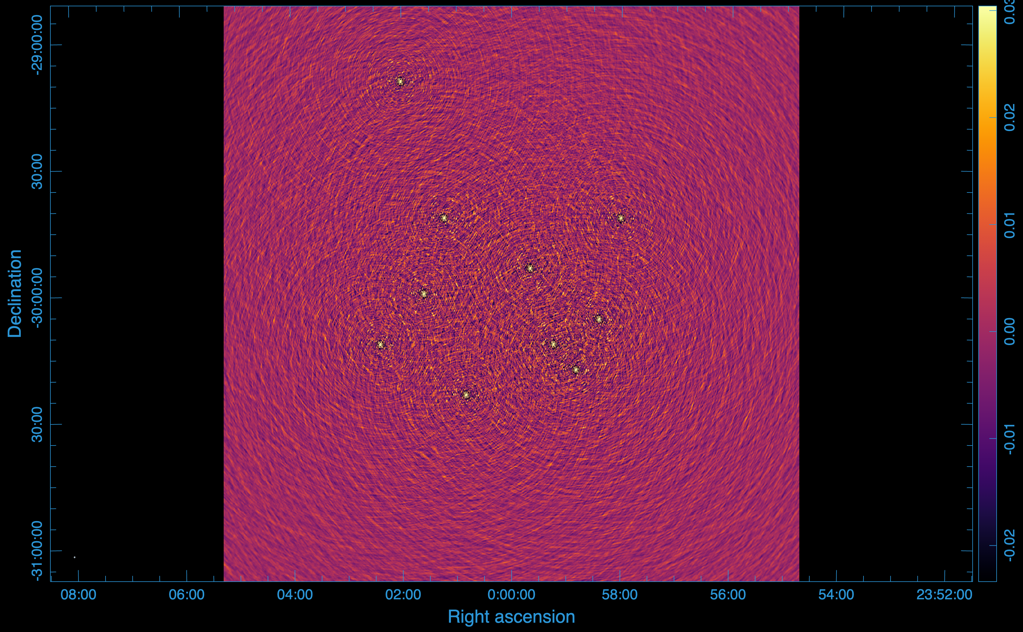
Statistics:
In this case, we will use the source furthest from the phase centre.
Peak flux: (\(9.897630810738 \times 10^{-1}\)) Jy/beam
RMS: (\(1.888134699183 \times 10^{-2}\)) Jy/beam
SNR: 52
Disk usage:
The MS occupies 43 GB of disk storage.
Compression using first singular value#
The compression for the MeerKAT telescope is extremely computationally expensive as there are 2016 baselines, so we add the –batch-size flag, which let us decide the number of the baselines to process at the same time. We still choose to compress using the first singular value.
visco compressms -ms meerkat-sim.ms/ -zs meerkat-sim.zarr -col DATA -corr XX,XY,YX,YY -cr 1 -nw 8 -nt 1 -ml 4GB -da 2727 -csr 10000 -bs 200
where:
-bs determine the batch size or the number of baselines to process at once.
Data image:
After compressing the data using only the first singular value (compression rank of 1), we get this image:
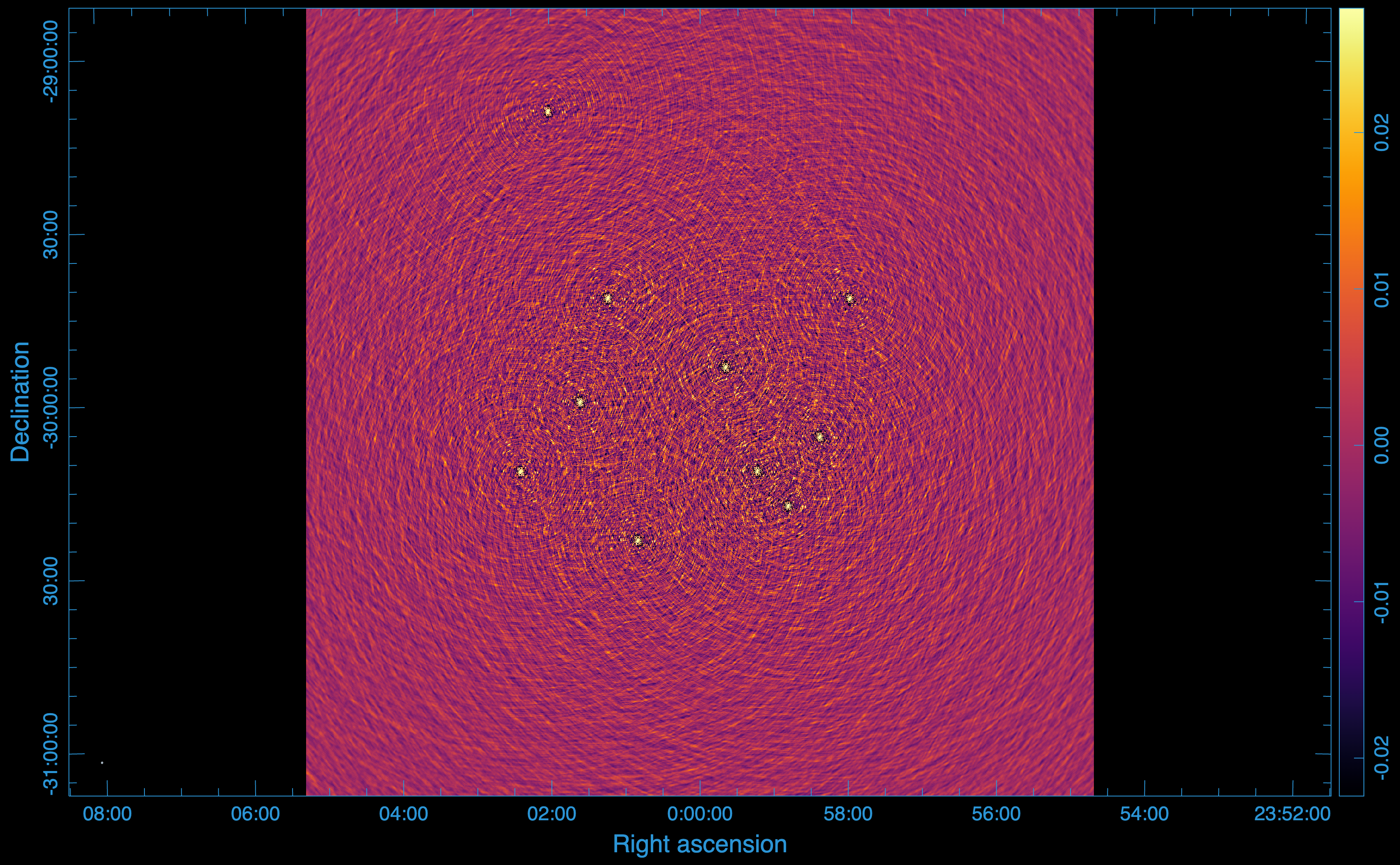
Statistics:
Looking at the image produced after the compression, there is no visible difference. However, going back to the furthest source from the phase centre, we get:
Peak flux: (\(5.085088610649 \times 10^{-1}\)) Jy/beam
RMS: (\(1.192684202182 \times 10^{-2}\)) Jy/beam
SNR: 34
Smearing:
After compression with the first singular value, only 51% of the peak flux is recovered on the source furthest from the phase centre. This demonstrates that in this case, the first singular value is not sufficient to fully retain or recover the signal. Consequently, we must use more singular values (higher compression rank) in the compression.
Disk usage:
The zarr store containing the compressed data only occupies 1.2 GB of disk storage, representing a compression factor of 35.
Compression using the first 6 singular values#
Since compression using only the first singular value did not work, here we try to use the first 6 singular values (compression rank of 6). We only change our –cr flag on our run:
visco compressms -ms meerkat-sim.ms/ -zs meerkat-sim.zarr -col DATA -corr XX,XY,YX,YY -cr 6 -nw 8 -nt 1 -ml 4GB -da 2727 -csr 10000 -bs 200
Data image:
After compressing the data using the first 6 singular value, we get this image:

Statistics:
With the first 6 singular values, we get:
Peak flux: (\(9.898513555527 \times 10^{-1}\)) Jy/beam
RMS: (\(1.672275516698 \times 10^{-2}\)) Jy/beam
SNR: 52
Smearing:
After compression with the first 6 singular value, 100% of the peak flux is recovered for the source furthest from the phase centre. This means that the first 6 singular values are sufficient for the compression and to fully retain the signal.
Disk usage:
The zarr store containing the compressed data now occupies 2.2 GB of disk storage, representing a compression factor of 20.
Compression using the Decorrelation flag#
Instead of enforcing the same compression rank (singular values) across all baselines for compression, you can choose to apply variable compression rank for each baseline by using the –decorrelation flag. By specifying decorrelation level, the user specifies the minimum percentage of the signal that needs to be retained for each baselines. This is the recommended method, especially if you are dealing with low signal-to-noise ratio (SNR) sources, as applying the same compression rank across all the baselines leads to significant smearing effects on long baselines. Using this method is equivalent to using baseline dependent averaging (BDA) with SVD, resulting in short baselines being more aggressively compressed than long baselines. To use this, you can run:
visco compressms -ms meerkat-sim.ms/ -zs meerkat-sim.zarr -col DATA -corr XX,XY,YX,YY -dec 0.98 -nw 8 -nt 1 -ml 4GB -da 2727 -csr 10000 -bs 200
where:
-dec specifies the percentage signal to be retained for each baseline.
Data image:
In this case, we specified a decorrelation level of 0.98, which means that on each baseline, at least 98% of the signal will be retained. With this, we get the following image:

Statistics:
Peak flux: (\(9.897790551186 \times 10^{-1}\)) Jy/beam
RMS: (\(1.888192330344 \times 10^{-2}\)) Jy/beam
SNR: 52
Smearing:
There is no smearing since we chose a decorrelation level 0f 98%.
Disk usage:
Using the decorrelation method results in a less compression ratio. This is because more singular values could be used than needed. As a result, the zarr store containing the compressed data now occupies 12 GB of disk storage, with a compression factor of 4.
Note
The choice of compression rank or decorrelation level depends on the specific scientific goals and the acceptable level of data loss. Users should carefully evaluate the trade-offs between compression efficiency and data fidelity for their particular use cases.
Tutorial 4: Dealing with Flagged Data#
In real observations, some data points are often flagged due to various reasons such as radio frequency interference (RFI) or instrumental issues. visco can handle flagged data during compression using three different options.
Using a replacement value#
One way to handle flagged data is to replace the flagged visibilities with a specific value before compression. This can be done using the –flagvalue option. For example, to replace flagged data with one, you can run:
visco compressms -ms meerkat-sim.ms/ -zs meerkat-sim.zarr -col DATA -corr XX,XY,YX,YY --flagvalue 1+1j -dec 0.95 -nw 8 -nt 1 -ml 4GB -da 2727 -csr 10000 -bs 200
This command replaces all flagged visibilities with the complex value (1 + 1j) before performing compression. This approach is not recommended as it can amplify noise and introduce artifacts.
Using interpolation#
Another approach is to interpolate the flagged data points based on the surrounding unflagged data. This can be done using the –flagestimate option. For example:
visco compressms -ms meerkat-sim.ms/ -zs meerkat-sim.zarr -col DATA -corr XX,XY,YX,YY --flagestimate -dec 0.95 -nw 8 -nt 1 -ml 4GB -da 2727 -csr 10000 -bs 200
This approach estimates the flagged visibilities by first gridding the unflagged data and then interpolating to fill in the flagged points. This method is more effective, However, it can be computationally intensive.
Using MODEL Data#
A more robust method is to use the MODEL column in the Measurement Set to fill in the flagged data points. This can be done using the –use-model-data option. For example:
visco compressms -ms meerkat-sim.ms/ -zs meerkat-sim.zarr -col DATA -corr XX,XY,YX,YY --use-model-data -dec 0.95 -nw 8 -nt 1 -ml 4GB -da 2727 -csr 10000 -bs 200
This is the recommended approach as it leverages the existing model visibilities to accurately fill in the flagged data points, leading to better compression performance and reduced artifacts.